Double centroid line regression

I thought of this way to do a regression of points that is much simpler than the least squares approach, as that involves using the derivative to find a minimal arrangement.
First you have your data points:

Step 1: Find the centroid of the points. This is just averaging the x values and y values of all the points. There are 8 points here so I would add all the x values and divide that sum by 8, and add the 8 y values and divide by 8, to get a point x1, y1.
Step 2: Find the centroid of every point with an x coordinate greater or equal to x1. Here there are 6 points on the graph to the right of x1,y1. So I would sum the 6 x values and divide by 6 and sum the 6 y values and divide by 6. This gives x2,y2.
Step 3: Create the line connecting x1, y1 and x2,y2. Line(T)=x1*(1-t)+x2*(t), y1*(1-t)+y2*(t), for t from a to b, you can choose a and b to make the line as long as you want.
This gives C:

This is your regression. 

Theorem: This line C balances the points on either side of C. 

Proof:You know the left and right sides with respect to x1,y1 balance because x1,y1 is the centroid. x2,y2 is the centroid of all the points to the right or above and below x1,y1.Imagine another point x3,y3 that is the centroid of all the points to the left or above and below x1,y1. x2,y2 and x3,y3 must balance across x1,y1 because x1,y1 is the centroid and all other points balance at either x2,y2 or x3,y3.. This means there is a line through x1,y1, x2,y2, and x3,y3 because if they weren't collinear x1,y1 couldn't be the centroid of all the points.  That line must have the property that the centroid of the points on one side of the line reflect across the line to the centroid of the points on the other side of the line because it passes through the 3 centroids balancing all the points.  

Theorem: This line C has the shortest total of distances squared to the points as measured by the length squared or quadrance of segments from C to all the points, each perpendicular to C.

Proof: Mirror all the points across C making pairs of points adding new points as necessary, C is still the line of balance because the midpoints of all those pairs still lie on C. This doubles the total distance squared to all the points.  Then move every point so they all have the same distance squared to C as the average distance squared to C, this doesn't change the total distance squared and C still balances the points because the midpoint of every pair hasn't changed. For every pair of points, the distance to each from C is the same: a. This minimizes the sum of the distances squared to the two points ,  because if move the midpoint that is on C, to still balance the points it must be on the line connecting the two, but if we lengthen one distance and decrease the other both by c, to maintain the total distance, we have
(a+c)^2 + (a-c)^2 > 2*a^2
because
a^2+c^2+2*a*c + a^2+c^2-2*c*a > 2a^2
because
2(a^2 + c^2) > a^2
for any choice of c .
So since we can only increase the sum of the distances squared to C in this way,  the point on C minimizes the distance squared to each pair of points, which means it minimizes the distance squared to any subset of these points because they all have the same distance squared to C. And the original points are a subset of these points so C minimizes the sum of the distances squared to them.

Comparison to Least squares method on sample data
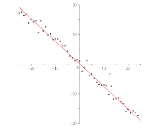
On here is using Maple's least square method vs. the data:

Maple said the linear function should be -.762*x+1/1000.
Here is using this method I made:

My method said the function should be .76*x + .15 (after solving the parametric equation it yields for y in terms of x). So the solutions are both really close but mine ended up a little closer to the function I used to generate the data, I used .75*x+.25 and then added a random amount by picking a random number from a normal with mean 0 and variance 1.

The advantage to using mine versus the standard is that mine is simpler to compute running in linear time vs. the standard method has to solve a matrix which can run in somewhat less than O(n^3) time, so it is much faster taking only the cube root of n as much time.  My method doesn't require the points to be one to one with the x-axis, and because it uses a parametric equation the best fit to the data could even be a vertical line whereas that would break the usual method.  The axioms needed to use my method are simpler to explain as they only involve basic geometrical ideas and not calculus. And at least in this one test it gave a better approximation of the data than the usual method. I can't think of any disadvantages...