DC to 60 hz AC square wave converter

Above: Red, black, green and purple are copper electrodes, copper colored is two separate pieces of solid copper, and blue is non-conductive material.
First the solid copper parts are fitted together with the non-conductive part. I'll call these two together the Axel. Here are what the two opposite sides look like, note the copper sticks through the insulation on the lower half in two rectangular shapes, I'll call these the lower and upper notches...

Then the electrodes are held in place around the outside of it like so:

The red piece is connected to the negative terminal of the DC source electricity. The black piece is connected the positive terminal of the DC source. The green and purple electrodes are the square wave AC output electrodes. Then, with the electrodes held fixed in place, the Axel is made to spin around it's long axis inside the electrodes. This is accomplished by mounting the Axel on a 3600 rpm DC motor.

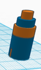
The upper notch as I've named it alternates between touching the red and the black DC electrodes, as the lower notch is touching the opposite electrode. As the Axel spins the notches stay in contact with their respective electrode for about half a revolution. The lower notch has a direct electrical connection to the purple electrode, and the upper notch is directly connected to the green electrode. Thus the purple and green electrodes are switching polarity at 3600 times per minute, or 60 hz at the same voltage as the DC source, hence the output is an AC square wave.

Smooth step sum of functions

This function is all operations in base 2 for ease of calculation on a computer...

h is the height and a is a point on the x-axis, like below for height for at a=3...

It's nearly flat on top, and at half a unit away in either direction it is one quarter of the full height, which makes it so when you put it next to another function of the same type, the point halfway between them is halfway between the height of both... There is negligible height anywhere outside of [a-1...a+1]

the leading coefficients in the above are 2,5,-1,3,2,5 so those are the heights for a = 0,1,2,3,4,5

solar distiller

I made like five or six improvements to my solar distiller idea... it was hard to get a good picture of the shape of the plastic lid, the bottom is like a square pyramid shape so it slopes to the center from every side, and the top of it has that same shape cut into it, so a bunch of lids could stack all together and it also acts as a lens aiming the sunlight from overhead more onto the area where whatever is being heated is. I think it would be pretty good for doing something like making raisins from grapes as well...

Integral estimate from many short quadratic functions...

The end result is:

The reasoning is, suppose you have your function f(x) and a point a, then these two functions are close to equal around x=0 for smaller and smaller values of d...

The bottom formula M is just the second degree Maclauren series of f(x-a) using divided differences for the first and second derivative..
So for example:

The red function approximates sin(x-.75) around 0
So to find the area of sin(x) from let's say [x-d... x+d] we can integrate M with respect to x instead:

Then evaluate this integral from x-d to x+d with x = 0.

That simplified nicely! 

Now to do a whole interval we can just do the sum of this above function over the interval but that will count all but the very left and very right interval twice as [x-d..x+d] and [x-2*d..x] overlap the [x-d..x] region and the same on the right side of x, but either one quadratic function will be an overestimate and the other an underestimate or they're both overestimates or they're both underestimates any of which case the average is better than the worst of the two, so we divide by 2 after all is done and that minimizes the error overall, this is an oversimplification, but correcting for the far left and far right interval only being counted once adds complication for not much gain, and the error when d is small is small.

And that's the given formula... for example [.5..3] for sin(x) and d=.01 :

for d = .001

**Comparison with other methods**
Other than the fact that the above example is a periodic function which the trapezoidal rule tends to work for really well, for other classes of functions it should be much better than the trapezoidal rule for approximately the same amount of computation because it fits closer to the real curve... It compares to the Simpson's rule that it is quite like doing the Simpson's rule over many small intervals and adding the results together. Since the Simpson's rule uses a quadratic function over the entire interval and this uses many smaller quadratic functions over the interval, so it is more accurate in general, though Simpson's rule is faster to compute.
**Extensions**
It would be pretty straight forward to extend this to many small cubic, quartic, etc.. approximations over small intervals.

solar distiller

I built this to distill dirty water into clean water, you put the 2-liter of bad water into the receiver which is made out of the top of a Styrofoam cup and duct taped into place. The water fills the pan in a shallow layer with a lot of surface area for better exaporation.  The bottom of the pan is arched so the water level never reaches the whole cut in the bottom that is fitted with a cut off top of a 2 liter, the water exaporates inside the pan in the sun and collects on the plastic covering which is weighed down in the middle so the water runs down it and drips through the cut off 2 liter top which acts as a funnel. This water is collected into another empty 2 liter that screws onto the cut off 2 liter on the underside with a female-female 2-liter adapter (two 2 liter caps duct taped together lol) and the pan sits on four legs to hold it steady.

I think there could be a manufactured version that has the pan, the funnel and hole in the bottom, the receiver and legs all built out of a single piece of metal, with a fitting plastic lid of the right shape, so all you would need to use it is a 2 liter of dirty water and a clean 2 liter to store the water...

Accurate estimation of arclength

To show the basic principle with a simple example, let's start with x^2 from 0 to 2:

One could use the arclength formula to find the arclength of course:

But an alternative I thought of was to use polynomial interpolation on the arclength f ( square root of 1 plus the derivative squared) and integrate to get:

The reason to use this instead is if you consider more complex curves like:

If you tell Maple to figure this arclength from [-3..1] it will just sit there forever churning unable to do it. So normally you would have to do a kind of sum of straight line approximations along the curve, but If you break the curve into manageable pieces you can use this method I'm proposing. I'll choose the interval [-3..-1] because it's always increasing there, f is square root of 1 plus the derivative of the above function squared ...

I found that 5 point polynomial interpolation is good for getting very close to the correct answer while being very fast to calculate, but if more accuracy was needed or more speed the number of points in the interpolation could be varied. 

**Edit***

I think another approach would be to just break the curve into a certain number of equal parts and then use 3 point interpolation on those pieces, which would be a quadratic Simpson's rule which leads to coefficients like this:

You would sum this over the interval for a certain d diminishing for more accuracy, but apparently never 0 because d is in the denominator.

Pick's Theorem and Gauss's Circle problem

Gauss's circle problem asks a question that at it's heart concerns how many integer lattice points are inside or on the circle on a grid:

Above if you counted them all there would be 113.
For a close estimate I did the following:

Here I've drawn a shape that is only 4 away from containing every lattice point inside or on it's boundary. 

It's perimeter has to be (r-1)*8, above for r=6. Because you eventually will have gone up 5*2 times down 5*2, right 5*2, left 5*2... which is 5*8. 

You can see that the area of the red figure should be somewhere between pi*5^2 and pi*6^2 because it lies between both circles at all times. 

So for a figure like the red figure we can use Picks theorem to figure out the number of points inside and on the boundary of the red figure...

This relates the area, which we will approximate, the number of interior points i and the number of boundary points.

So for our red figure the estimate works out to:

So for example, a circle with radius 46 would have around 6683 by this estimate, the actual value is 6625 so the estimate is within 1%.
**Note** it's also possible to figure absolute upper and lower bounds by using the outer or inner circle, the estimate above just averages the lower and upper bound together...
I only showed for the circle, but the general idea could apply to ellipses or other shapes with known areas or number of lattice points under a curve, etc...

Slow but dense poisson disc distribution sampling

The idea for this algorithm is to somewhat randomly place many dots that are all at least a certain distance apart, without placing so many that it becomes hexagonal close packed packing which is the densest possible. It ends up looking a lot like how the light sensitive cells are arranged on the retina.
This algorithm is slow but has a good end result here it is for 200x200 no two closer than 5 units apart:

The algorithm makes a list of every single possible pixel value shuffled in random order F, then starts with a field with only one random point on it p of list P, pops the first value v off of F and adds it to P if the distance from v to any point p in P is greater than d, where d is the minimum distance between points. The algorithm stops when there are no longer any values in F. In the above at the end there were 2337 points in P.
**improvements?**
I could add logic so the points are on a toroidal surface with the top and bottom attached and the sides attached, also if all the points p in P were stored in an octree type structure I think there could be some good performance gains.

**Python Source Code**
import random
from random import shuffle
import Image
def fill(grid, sizegrid):
    for i in range(0, sizegrid[0]):
        for j in range(0, sizegrid[1]):
            grid.append([i,j])
    shuffle(grid)
def distance(pointa, pointb, mindistance):
    if abs(pointa[0]-pointb[0]) >= mindistance:
        return mindistance+1
    if abs(pointa[1]-pointb[1]) >= mindistance:
        return mindistance+1
    return ((pointa[0]-pointb[0])**2 + (pointa[1]-pointb[1])**2)**.5 
def plot(points, sizegrid):
    p = Image.new("RGB", sizegrid)
    for i in points:
        if i[0] >= 0 and i[1] >= 0:
            p.putpixel(i, (255,0,0))
    p.save("out.png")
def add(a, points,mindistance):
    for point in points:
        if distance(point, a, mindistance)<mindistance:
            return False
    points.append(a)
    return True
def main():
    sizegrid = (200, 200)
    points = [[random.randint(0, sizegrid[0]-1), random.randint(0, sizegrid[1]-1)]]
    fullgrid = []
    fill(fullgrid, sizegrid)
    mindistance = 5
    while(len(fullgrid) > 0):
          f = fullgrid.pop()
          if add(f,points, mindistance):
               points.append(f)
    plot(points, sizegrid)
    print(len(points))
main()