within 6% Vector Coordinate Interpolation

For n points in any number of dimensions with coordinates P(n),

The function above interpolates the points within an error range of about 6% of the magnitude of the vector to each point... P(0) in the graph below is A, P(1) is B, up to P(6) being A again...

The above is 5 points of 2d vectors being interpolated... The nice thing about this formula is it applies to any number of points in any number of dimensions...

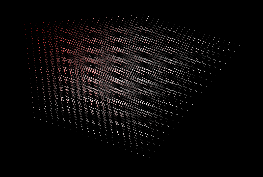
It goes very nearly through the midpoints between each pair of successive vertices, I think changing the e values in the formula to possibly two different numbers might be able to close in closer to the given points but maybe at the expense of not going as nicely through the midpoints...

The term inside the sum multiplying with the point vector is a normal distribution, with a value of 1 at a particular integer t value and tapering off on each side so that it's roughly 1/2 at the half integers on either side. The ideal would be a distribution with a peak of 1 at an integer t value and a value of exactly 1/2 at each half integer on either side and going completely to 0 everywhere at the integers on either side and beyond, but I think that's only really possible to approximate with a closed form function... Also if you go all the way to a triangular distribution over the interval so you make perfectly the polygon including the points you lose the nice property that the derivative is defined continuously everywhere...

Vector Coordinate Parameterized Ellipse in Triangle

The traced curve varying t goes through the midpoints of the sides of the triangle...

sphere to modular plane

I was thinking some problems that take place on a sphere might be easier thinking of them on the modular plane and some modulo problems might be easier thinking of them on a sphere...

Point in convex polygon by coefficients times vertices

Supposing you have n vertices in the plane forming a convex region chosen to be indexed in some order by i, I found that any point inside that convex polygon can be expressed as the sum of coefficients [0..1] multiplying each vertex with coefficients adding to 1...

For example if the vertices were V[0], V[1], V[2], V[3], V[4], a point inside the polygon will be 

.2*V[0]+.4*V[1]+.2*V[2]+.1*V[3]+.1*V[4]

Note that the coefficients add to 1 and are between inclusive 0 and 1!

I wrote this program to demonstrate. This is plotting points for any coefficients meeting these two criteria in 20 discrete steps between 0 and 1 inclusive and 5 vertices...

I've made it so c[0] makes a plotted point redder proportional to how large the coefficient is...

Below is with 50 discrete values between 0 and 1 of the variables:

I think it's clear with fine enough steps every part of the pentagon would be plotted, perhaps uniquely...

I'm still working on a proof though... I wrote the program just to see if it obviously wasn't true but it looks like it is...

**Source Code requires Python 3 and Pillow for Python**

from PIL import Image

def descend(n, c, i, s, d, plot, coords):

    if i < n-1:

        m = 1.0

        while(m >= -d/2.0):

            c[i] = m

            if(s+m <=1-d/2.0):

                descend(n, c, i+1, s+m, d, plot, coords)

            m -= d

    else:

        c[n-1] = 1.0-s

        print(c)

        p = [0,0]

        for j in range(0, n):

            p[0] += c[j]*coords[j][0]

            p[1] += c[j]*coords[j][1]

        plot.putpixel((int(p[0]), int(p[1])), (255,255-int(c[0]*255),255-int(c[0]*255)))

        

def main():

    coords = [[84,232],[104, 424],[342,508],[528,276],[330,212]]

    plot = Image.new("RGB", [800,800])

    c = [0,0,0,0,0]

    descend(5, c, 0, 0, .05, plot, coords)

    plot.save("plot.png")

main()

recursive cosine square wave?

This recursive function might eventually go to a square wave...

feathery function

Parallel convex hull algorithm #2

So supposing you have points on the plane with known coordinates...:

First find the centroid (marked in red) and the four points with extreme values of x and y coordinates...

Any point inside the triangles formed can be removed...

Now the recursive step is to find from the centroid  lines dividing each triangle into two pieces such that the point the line ends on is the farthest from the centroid within that section like so:

Now form triangles and remove points again...

In this case we were already done with thte last lines added forming the convex hull...

But the process may need to be iterated until all remaining points are on the polygon...

It may be useful to use polar coordinates centered at the centroid then the points can be sorted by theta and easily split into sections and the furthest point would be the point with the largest r value in each section...I think it should then be fairly straightforward to extend it to 3 dimensions using spherical coordinates instead...

Notation for Direction and Distance plots on Cartesian plane

I will be considering these two formulas which are good for modelling a situation when you know the angle you want the plot to go in with respect to the x axis from a point and how far in that direction for each of n discrete steps...

With the meaning that X(n), Y(n) is the nth point in a series...

And to show with an example first let L(i) = i and theta(i) = i*2*pi/5

Interestingly Maple knew the closed form, but it's not necessary for a limited number of points, it does make it easy to plug in any value of n and find the point without knowing any of the previous points though... 

And we can make a list over n=1, 2, 3,4,5

And we can let the initial point be [0,0] to get:

An then plotting the above, both with natural number n and continuous n:

In general L(i) can be any discrete function of length of lines for the plot and theta(i) can be any function for the angle the lines make with the x axis...

**Next is to see what happens when L(i) is a constant with a delta->0 length and theta(i) gets more continuous