spiral chart

A program I wrote takes some values like:
[3,5,2,8,1,3,7]
first sorts greatest to smallest:
[8,7,5,3,3,2,1] (The program works whether they are sorted or not)
Then makes a spiral with the area of each rectangle corresponding to the values in this list... it doesn't write the numbers on them but I've labeled them:

I had intended it as a good way to show the relative sizes of elements of a dataset, but it doesn't really work for that as well as I thought it would because I think people aren't as good at recognizing rectangular areas and there's some optical illusions.
For example:
[1,1,1,1,1,1,1]

I had to actually measure these to verify they all have the same area so that precludes it from being a good tool for data representation. It's kind of an interesting optical illusion though.
The way I wrote the program you can put any size in for the main rectangle here is the all 1's again but in 800x350

There can be any number of data points here is 14 following the Fibonacci series:

This one is a 1920x1080 for a desktop background of the numbers 1,2,3,...13,14

I'm kind of proud of this source code, it took some thinking to make the program this short...

*Python Source Code**
import Image, ImageDraw
def rsum(data, i):
    sum = 0
    if i+1 < len(data):
        for d in range(i, len(data)):
            sum+=data[d][0]
        return sum
    else:
        return data[len(data)-1][0]
def parserec(coords):
    leastx = coords[0][0]
    leasty = coords[0][1]
    mostx = coords[0][0]
    mosty = coords[0][1]
    for i in range(1, len(coords)):
        if coords[i][0] < leastx:
            leastx = coords[i][0]
        if coords[i][0] > mostx:
            mostx = coords[i][0]
        if coords[i][1] < leasty:
            leasty = coords[i][1]
        if coords[i][1] > mosty:
            mosty = coords[i][1]
    return [(leastx, leasty), (mostx, mosty)]
def main():
    size = [800,800]
    pic = Image.new("RGB", size)
    draw = ImageDraw.Draw(pic)
    data = [[1, (255,255,0), "widgets"],[1,(255,0,0), "thingies"],[1,(0,255,0),"stuff"],[1,(0,0,255),"foo"], [1,(0,255,255),"bar"], [1,(125,125,255),"bar2"],[1,(125,125,0),"bar3"]]
    r = rsum(data,0)
    data = list(reversed(sorted(data)))
    rects = [[(0,1),(0,0),(size[0],0),(size[0],1)], [(size[0]-1,1),(size[0],1),(size[0],size[1]),(size[0]-1,size[1])],[(size[0]-1, size[1]-1), (size[0]-1, size[1]), (0,size[1]), (0, size[1]-1)],[(1,size[1]-1), (0, size[1]-1), (0, 1), (1, 1)]]
    for i in range(0, len(data)):
        thisrect = i+4
        width = data[i][0]*1.0/rsum(data, i)
        x0 = rects[thisrect-1][3][0]+width*(rects[thisrect-1][0][0]-rects[thisrect-1][3][0])
        y0 = rects[thisrect-1][3][1]+width*(rects[thisrect-1][0][1]-rects[thisrect-1][3][1])
        x1 = rects[thisrect-1][3][0]
        y1 = rects[thisrect-1][3][1]
        x2 = rects[thisrect-3][0][0]
        y2 = rects[thisrect-3][0][1]
        x3 = (x0-x1)+x2
        y3 = (y0-y1)+y2
        coords = [(x0,y0),(x1,y1),(x2,y2), (x3,y3)]
        rects.append(coords)
        coordstlbr = parserec(coords)
        draw.rectangle(coordstlbr, fill=data[i][1])
    pic.save("spiralgraph.png")
main()

square angles (squangles)

First every vector in the plane can be mapped to the 2 by 2 square centered at the origin by dividing both components of the vector by the magnitude of the larger of the two components. So (3,6), the larger of the two components is 6 so divide both components by 6 and get (1/2,1), which is a point on the  square. For (-5,-2) the magnitude of the larger component is 5 so divide both by 5 and get (-1,-2/5) which is the corresponding point on the square. 

To find the angle between 2 square normalized vectors find the distance around the square to get from one coordinate to another. In this case from (1/2,1) you have to go left 1+1/2 and then down 1 and 2/5 to get -2.9 because you're going counterclockwise.  From the other vector it would be 2.9 clockwise.

It's an algorithm rather than a direct math quantity to find the square angle because of the complications first in finding the normalized square vector, that you have to divide by the largest component which is hard to put as a formula, and then in finding a formula for the distance around the square without using modular arithmetic or absolute values etc..., but it is nice that the angles around always add to 8,  squangle(a,b)+squangle(b,c)=squangle(a,c) and counterclockwise comparison is always a negative angle, etc...

**Note

I thought at first there would be a sort of distortion from the corners but there really isn't, consider the square angle between (0,1) and (1,0) and between (1,1) and (1,-1)  are both 2 even though one consists of just a straight line and the other goes around a corner. Any two vectors that the angle between them would ordinarily be 90 degrees the square angle is 2, 30 degrees 2/3 etc... This relationship makes it possible to use the algorithm to find the square angle, then convert to the regular angle without having to ever use a trigonometric function like cosine.  I think a proof of that could be start anywhere as a normalized square vector, add the square angle to itself as many times as will fit in 8, that has to map exactly to an angle of a certain number of degrees added to itself as many times as it goes into 360 because either way you went all the way around. 

simple locating goal and finding short path to it algorithm

The red square can move to any white square but is blocked by black squares. It can only check whether the square it is on is yellow (the goal). So the object is for the red square to find the yellow square and return a reasonably short path to getting there around obstacles and so on.
My algorithm is very simple, the red square keeps a list of squares he's visited, and randomly moves to another acceptable square by moving up,down,left,right, or any diagonal one square. Then he checks his list to see if he's ever been 1 move away from any square on his list starting at the beginning of the list. If he has been then he shortens his list by removing every square visited in between where he currently is and the earliest time he was 1 square away from where he is now. This has the effect of removing loops and double backs from the final path. This is like finding a "short cut" between where he is and where he was. Eventually he will end up on the yellow square and the program ends and returns his list.
**Python Source code
import Image
import random
class board():
    board = [[0,0,0,0,0,0,0,0,0,0],[0,1,1,1,1,1,1,1,1,0],[0,2,1,1,1,1,1,1,1,0],[0,1,1,1,1,1,1,1,1,0], [0,1,1,1,0,0,1,1,1,0], [0,1,1,1,0,0,1,1,1,0], [0,1,1,1,1,1,1,1,1,0], [0,1,1,1,1,1,1,1,1,0], [0,1,1,1,1,1,1,1,1,0],[0,0,0,0,0,0,0,0,0,0]]
    mousepos = [8,8]
    def drawboard(self, img):
        for i in range(0, 10):
            for j in range(0, 10):
                if self.board[i][j] == 1:
                    for m in range(i*50, (i+1)*50):
                        for n in range(j*50, (j+1)*50):
                            img.putpixel((m,n),(255,255,255))
                if self.board[i][j] == 2:
                    for m in range(i*50, (i+1)*50):
                        for n in range(j*50, (j+1)*50):
                            img.putpixel((m,n),(255,255,0))
                if self.mousepos[0] == i and self.mousepos[1]==j:
                    for m in range(i*50+10, (i+1)*50-10):
                        for n in range(j*50+10, (j+1)*50-10):
                            img.putpixel((m,n),(255,0,0))
    def drawsolution(self, img, states):
        for i in range(0, 10):
            for j in range(0, 10):
                if self.board[i][j] == 1:
                    for m in range(i*50, (i+1)*50):
                        for n in range(j*50, (j+1)*50):
                            img.putpixel((m,n),(255,255,255))
                if self.board[i][j] == 2:
                    for m in range(i*50, (i+1)*50):
                        for n in range(j*50, (j+1)*50):
                            img.putpixel((m,n),(255,255,0))
        for mousepos in states:
            for m in range(mousepos[0]*50+10, (mousepos[0]+1)*50-10):
                for n in range(mousepos[1]*50+10, (mousepos[1]+1)*50-10):
                    img.putpixel((m,n),(255,0,0))
                    
                        
    
class mouse():
    b = board()
    states = []
    def move(self, img):
        mousepos = self.b.mousepos
        okmove = False 
        while(okmove == False):
            tx = random.randint(-1,1)
            ty = random.randint(-1,1)
            if self.b.board[mousepos[0]+tx][mousepos[1]+ty] != 0:
                if self.b.board[mousepos[0]+tx][mousepos[1]+ty] == 2:
                    print "Found cheese"
                    print self.states
                    self.b.drawsolution(img, self.states)
                    return True
                mousepos = [mousepos[0]+tx, mousepos[1]+ty]
                self.b.mousepos = mousepos
                okmove = True
        self.checkstate(mousepos)
        return False
    def checkstate(self, mousepos):
        print mousepos
        self.states.append(mousepos)
        
        for i in range(0, len(self.states)-1):
             if self.states[i][0] == mousepos[0]-1 or self.states[i][0] == mousepos[0]+1:
                 if self.states[i][1] == mousepos[1]-1 or self.states[i][1] == mousepos[1]+1:
                     print "shortcut"
                     states2=[]
                     for j in range(0, i+1):
                         states2.append(self.states[j])
                     self.states = states2
                     self.states.append(mousepos)
                     break
                    
                
def main():
    
    img = Image.new("RGB", [500,500])
    m = mouse()
    while(m.move(img) == False):
        pass
        
    img.save("mouseboard.png")
main()

somewhat generalized recurrence

I'm not sure what class of curves this works on, I've tried it on a few exponential looking curves.
Suppose you have 2*n numbers indexed to the counting numbers:

You'd like to know a logical way it could continue...

A graph of the series with where you might guess the next point would be if it follows a smooth curve is:

I found that you can project to a solution solving a set of n-1 equations of degree n-1 like so:

The points are in order 1,17,54,166,332,680. The first equation is set up so the last point is a^2 times the  point before it plus b times the point before that and 1 times the point before that. And this same type of recurrence is applied for the second equation to 332. 

So you solve for a and b and plug the values of those coefficients in for a next term 

x= a^2*680+b*332+166

 1442

So now the plot with that point added looks like:

It seems to fit well. 

**Edit

In the above I was using exponents on the coefficients, but since each variable only occurred to the same power I think it's sufficient to just eliminate the powers. And I was always just plainly adding the last term but it works out nicely that every point in the whole list counts in the calculation if that last term has a coefficient as well and it should be more flexible as far as which curves can be evaluated. 

For an even number n points in a list of L values at the counting numbers solve n/2 equations in n/2 unknowns with x being the n/2th letter of the alphabet like:

L[n] = a*L[n-1]+b*L[n-2] + ... x*L[n/2]

L[n-1] = a*L[n-2]+b*L[n-3]+...x*L[n/2 -1]

...

L[n/2+1] = a*L[n/2] + b*L[n/2-1] +...x*L[1]

Then use those coefficients to find the next point... 

List correlation metric

Suppose you have two lists of the same n items ranked according to two different different metrics. If they end up listing the teams in the same order, you could say that the metrics are correlated 100%. If they ended up listing the teams in the exact reverse order of each other then that could be -100% correlation...
So this formula gives 100% and -100% in those two extreme cases and also a value to every intermediate case.

Where P[i,1] and P[i,2] are the position of item i on list 1 and list 2 respectively. 

The part in red sums the squares of the difference between where each item appears on list 1 and where it appears on list 2. The blue part is what the sums of the squares of the differences would work out to if the two lists were in complete reverse order from each other, which also is the maximum the part in red can reach. So the red part divided by the blue part is a number from 0 to 1 where 0 is the two lists are in the same order and 1 is for when the two lists are in reverse order from each other.  
The rest reverses and scales the result between -100 and 100 with -100 being the lists are in reverse order to each other and 100 being the lists are in the same order, with perhaps many values in between.
**Example

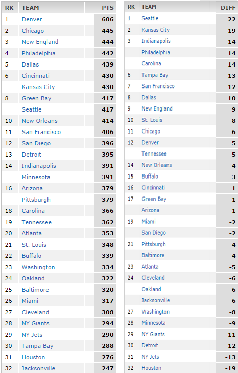
Consider the same graphic which lists how many points a football team in the NFL scored over last year and the difference between the number of turnovers they gained and how many they lost.

First we go through every team, and sum the squares of the differences for where they appear on each list. For example, the Denver Broncos are number 1 on the left list and 12 on the second so that is (12-1)^2=121. We do this for every team and add them all. The sum over all is 2298, and the blue part (an n of 32) of the formula is 10912, so plug those in the formula to get a correlation score of 57.8%, which is well towards a positive correlation on the scale of -100..100 so over a season a higher turnover differential correlates well with a higher point total.

** I think the nice thing about this method is it should detect any type of correlation, not just linear, because it doesn't depend on the values of the variables themselves just the order...  I think this would be a good initial test for any type of correlation and then you would use the conventional methods for determining which type of correlation, log normal, linear, etc..

Honeycomb coordinates

The basic idea is to traverse the honey comb grid. Going up is adding to an i component, going down and right is adding to a j component, and going down and left is adding to a k component, and if you go down, up and left, or up and right, it is -1 times the i,j,k components respectively.
For example consider the black path one unit at a time:
You go up:
1,0,0
Up and right:
1,0,-1
Up:
2,0,-1
Up and right:
2,0,-2
etc...
2,1,-2
2,1,-3
2,2,-3
1,2,-3
So the final coordinate is 1,2,-3
Now consider the red path:
0,0,1
-1,0,1
-1,1,1
-2,1,1
-2,2,1
-2,2,0
-1,2,0
-1,2,-1
-1,3,-1
-1,3,-2
-1,4,-2
-1,4,-3
0,4,-3
0,3,-3
1,3,-3
1,2,-3

You still end up at 1,2,-3!

So it's kind of interesting to consider which coordinates are actually possible, for example -1,0,0 isn't possible to reach from the starting position's type of vertex in the above picture, but it is starting from the other type of vertex. I notice the possible coordinates are 0,0,0 and every other coordinate's components sum to an odd number for either type of starting vertex.

Spectrum x Spectrum Blend

I made the plot above by averaging the color from the spectrum on the x axis with the one on the y axis, and as you see in the circled portion blown up you get some non spectrum colors such as brown. I don't know if this is every fully saturated color or if you get more colors adding another axis...
I'm thinking if you have two prisms shining their rainbow on a piece of white paper, there might be a way to hold them so their rainbows cross to make every color...
I'm not sure the cause of the roughly 3x3 grid that appears, whether that is because humans have 3 color receptors or because computers add 3 colors of light to make every color or both...

2,2,2 smooth curve source code

The main difference between this and Bezier curves or Nurbs is this doesn't use control points to guide the curve, it just goes through the points given directly. The way it does it is given 4 points it finds the best quadratic fit through the first 3 points parameterized from t=0..2 and the best quadractic fit for the last 3 points taken in reverse order parameterized from t=0..2 and makes a new point at the average of both curves at t=1.5. Then it does that for every group of 4 points to get twice the number of points, and recurses until it reaches the required resolution... 
The source code below takes for example these points:
points = [[50,300],[190,210],[344,256],[446,384],[580,294],[510,115]]
and generates a smooth curve through them in constant time with respect to the final number of points in the curve as described in the blog post before this...
here's a plot of the points, y increases as you move down because in image programs that's how they arrange the axis for some reason.

After the first iteration we find points between those given:

second iteration:

third:

After 10 iterations:

**Runtime complexity**
The program runs in constant time vs the final number of points generated.
**Source Code(Python) This source code requires PIL image library for python 2.7**
import Image
def e(coeff, t):
    return coeff[2]*t**2 + coeff[1]*t+coeff[0]

def m(a,b,c,d):
    coefflx = [b[0], -.5*a[0] + .5*c[0], .5*c[0]+.5*a[0]-b[0]]
    coeffly =  [b[1], -.5*a[1] + .5*c[1], .5*c[1]+.5*a[1]-b[1]]
    a,b,c
    d,c,b
    coeffrx = [c[0], -.5*d[0] + .5*b[0], .5*b[0]+.5*d[0]-c[0]]
    coeffry =  [c[1], -.5*d[1] + .5*b[1], .5*b[1]+.5*d[1]-c[1]]
    Xl = [e(coefflx, .5), e(coeffly, .5)]
    Xr = [e(coeffrx, .5), e(coeffry, .5)]
    return [.5*(Xl[0]+Xr[0]), .5*(Xl[1]+Xr[1])]
def n(a,b,c, side):
    coeffx = [b[0], -.5*a[0] + .5*c[0], .5*c[0]+.5*a[0]-b[0]]
    coeffy =  [b[1], -.5*a[1] + .5*c[1], .5*c[1]+.5*a[1]-b[1]]
    if side ==0:
        return [e(coeffx, -.5), e(coeffy, -.5)]
    else:
        return [e(coeffx, .5), e(coeffy, .5)]
def twotwotwo(plot, points, iter):
    points2 = [points[0], n(points[0], points[1], points[2], 0), points[1]]
    for i in range(0, len(points)-3):
        points2.append(m(points[i], points[i+1], points[i+2], points[i+3]))
        points2.append(points[i+2])
    points2.append(n(points[len(points)-3], points[len(points)-2], points[len(points)-1], 1))
    points2.append(points[len(points)-1])
    for i in points2:
        plot.putpixel((int(i[0]), int(i[1])), (255,255,255))
    plot.save("plot"+str(iter)+".png")
    return points2
def main():
    plot = Image.new("RGB", (640,640))
    points = [[50,300],[190,210],[344,256],[446,384],[580,294],[510,115]]
    for iter in range(1, 5):
        points = twotwotwo(plot, points, iter)
    
main()

2,2,2 Interpolation

Suppose you have a set of points and you want to find a smooth curve through them.

The dashed line is a sort of guess what it might look like, one of the points on it will be X somewhere between B and C.  First we find a parametric curve through points A,B,C called P[L,x] and P[L,y] with respect to t.

solve the above equations for the coefficients...

Plug these values for the coefficients back in the original equations...

Now plug in the actual values for A,B,C from the plot...

Let's look at the graph again...

So now for point X we consider the parametric equation going from D to C to B called P[R,x] and P[R,y] of t. The L and R are considering approaching point X form the left and from the right now as you can see. 

skipping a couple steps because it works the same the relevant part is...

and similarly

Now point X should be the average of t=.5 on all the P equations...

So we've found X...

All the points except between A and B and between E and F are found the same way. For the point between A and B we just have to use t=-.5 on P[L,x] and P[L,y] because that's the best information we have.

So once we've found all the points we'll have roughly twice as many points for our smooth curve, now we can repeat the process again on our new set of points and keep doubling the number of points until the curve is completely filled in down to the resolution we want.

**about the name**
I called it 2,2,2 interpolation because it uses a set of 2 2 dimensional parameterization's of degree 2 that are averaged to give 2 times the number of points. I suppose it could be taken to 3,3,3 and so on...