Rectangle billiard solution

Suppose you have a table and a linear paramterization for a ball on the table...

These equations tell you where on the table you'll be after time t, if the ball is thought to bounce off the walls as on a billiard table, where X and Y are the width and height of the table.

So it's interesting that with these equations, one can calculate directly the x,y position of the ball at, say,  time = 12845 without figuring out where it was at every time before that. 

Here is a plot of one example:

There is a field called dynamical billiards that studies more complicated ones, but for some reason they didn't give this nice solution to the rectangular one on wikipedia: http://en.wikipedia.org/wiki/Dynamical_billiards, I guess physicists are more interested in the ones that become chaotic.

complex angle

Consider the following, you first go 6 steps in the 1 direction and then 3 in the i direction:

So you divide the corresponding complex number by the total number of steps to get the complex angle.  Note that any similar triangle to this one in the same quadrant, like say (10+5*i)/15 equals the same complex angle. Also note that the complex angle preserves the quadrant the triangle is in. For negative x and positive y, for example, the complex angle will always be of the form -a+b*i, and so on for the four quadrants. 

bank shot

I read about this on a pool site but they didn't have a picture so I made this one, you aim for the reflected pocket on an imaginary pool table lying beside the one you're on to make the bank shot...

Tell whether a point is inside a polygon by reflection

I noticed if you have a convex polygon like so:

You can reflect this polygon across a point, in this case G...

And anytime G is outside of the original polygon, the polygons won't intersect...

But if G is inside the original polygon the reflected polygon will overlap:

So since there is an easy way to tell whether two lines intersect, one can look pairwise at every line and check for intersection to find whether g is inside the original polygon. It should also scale easily to 3 dimensions.
**EDIT**
A much faster way computationally than checking every pairwise intersection as I mentioned before, is to take your polygon with centroid marked as F:

Reflect across the test point G as before:

Now consider the parameterization of the line from F to F(1), if that line crosses a line in the original polygon first, then G is outside of the polygon. Or conversely:

If the parameterization crosses a line in the reflected polygon first or does not cross a line from either polygon as, G is inside the original polygon. If the parameterization is in terms of S, this would mean the crossing with the original polygon has a higher S value.  This takes the algorithm from having to check intersections of N^2 lines to just 2*N.

Beta sub t, binary comparison between x and y

I've defined this function:

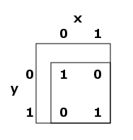
Where x and y are binary variables. And mod indicates the remainder of it's first argument when divided by it's second. The interesting thing about this function is to consider a certain truth table between x and y:

This could be considered !(x xor y) in the usual computer terminology, thought that starts to show how confusing the naming can be.
To see what Beta(t) does first look at the truth table read across as rows 1 0 0 1, this is the binary number 9, so we have:

First look at the function at x=0 and y = 0, the percent sign means maple uses the last result in place of the percent sign:

In general this Beta function at t produces the 0-15th truth tables for comparing x and y.  So to get the truth table that reads across by rows as 1 1 0 0, that is 12 in binary so you would look at B(12) at x = 0..1 and y = 0..1

**Explanation**

Note that the function in x,y over x=0..1 and y=0..1 is:

19*t+19 for t = 0..15:

19

38

57

76

95

114

133

152

171

190

209

228

247

266

285

304

These numbers above mod 17

2

4

6

8

10

12

14

16

1

3

5

7

9

11

13

15

Then the above mod 2:

0

0

0

0

0

0

0

0

1

1

1

1

1

1

1

1

The other four squares in the matrix go 0000111100001111, 0011001100110011, and 0101010101010101

so you get every combination in order...for example the 13th place in each of these four binary numbers is:

1,1,0,1 or 1101 which is the number 13 in binary...

modular additive network

Suppose you have a graph like the following:

I first fill in some starting values for all the nodes:

Call this State 1. State 2 is generated by adding the values of all nodes connected to a node and itself, then modding by a certain amount and adding 1. So if the mod amount is 7. The node with a 3 in state 1 would add 3+6+2 = 11, 11 mod 7 = 4, 4+1 = 5. so State 2 would have a 5 where the 3 is now.

It's interesting how long it takes to repeat the initial state, here are the first few States...
[2, 5, 2, 5, 6, 3]
[7, 1, 5, 5, 5, 5]
[3, 5, 3, 5, 7, 2]
[3, 3, 7, 7, 7, 6]
[7, 7, 6, 7, 3, 7]
[3, 7, 3, 4, 3, 3]
[7, 4, 6, 4, 3, 3]
[4, 1, 3, 5, 3, 6]
[3, 7, 4, 7, 1, 6]
[2, 1, 1, 5, 1, 5]
[4, 3, 4, 3, 1, 1]
[2, 1, 7, 5, 7, 7]
[2, 2, 4, 2, 1, 1]
...
This particular configuration repeated every 159 states. It's interesting that changing the initial values of all the nodes to some other number less than 8 for M = 7 still repeats after 159 iterations. Different M values repeat after different amounts of iteration, like M=11 repeats after 189...
source code:
graph = [[0,1,1,1,1,0],[1,0,1,1,0,0],[1,1,0,0,1,1],[1,1,0,0,1,0],[1,0,1,1,0,1],[0,0,1,0,1,0]]
amountsold = [7,5,3,5,4,3]
a = [7,5,3,5,4,3]
def add(graph, amounts):
    amountsnew = []
    for i in range(0, len(graph)):
        amount = amounts[i]
        for j in range(0, len(graph[i])):
            amount += graph[i][j]*amounts[j]
        amountsnew.append(amount%11+1)
    return amountsnew
print amountsold
for i in range(0, 1000):
    amountsold = add(graph, amountsold)
    if amountsold == a:
        print(i)

Alternative to Fourier Transform

I noticed if you have a plot, like this:

you can easily find some frequency information with this formula:

Where d is the number of divisions of the interval you want to analyze and r /d is the rightmost point... a slight modification could be made to shift the interval being analyzed from starting at 0. 

So for the values from the first image, with x of 100 and d of 10, if we vary s we get:

It appears the most interesting values are 2.5, 3, and 4.75... the original function I used to generate the data points was in fact:

The reason it works is pretty simple, no matter what your original wave is, if you add it together with a simple sine and cosine wave at a particular frequency and take the absolute value as per the formula, the result will be much larger on average over the interval if the original wave contains that frequency, as the waves "resonate" and reinforce each other making a larger value over the interval.
It seems much simpler than the Fourier transform, though it is somewhat less exact because there is noise in the result potentially making it more difficult to find the peaks.