Tell whether a point is inside a polygon by reflection

I noticed if you have a convex polygon like so:

You can reflect this polygon across a point, in this case G...

And anytime G is outside of the original polygon, the polygons won't intersect...

But if G is inside the original polygon the reflected polygon will overlap:

So since there is an easy way to tell whether two lines intersect, one can look pairwise at every line and check for intersection to find whether g is inside the original polygon. It should also scale easily to 3 dimensions.
**EDIT**
A much faster way computationally than checking every pairwise intersection as I mentioned before, is to take your polygon with centroid marked as F:

Reflect across the test point G as before:

Now consider the parameterization of the line from F to F(1), if that line crosses a line in the original polygon first, then G is outside of the polygon. Or conversely:

If the parameterization crosses a line in the reflected polygon first or does not cross a line from either polygon as, G is inside the original polygon. If the parameterization is in terms of S, this would mean the crossing with the original polygon has a higher S value.  This takes the algorithm from having to check intersections of N^2 lines to just 2*N.

Beta sub t, binary comparison between x and y

I've defined this function:

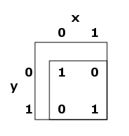
Where x and y are binary variables. And mod indicates the remainder of it's first argument when divided by it's second. The interesting thing about this function is to consider a certain truth table between x and y:

This could be considered !(x xor y) in the usual computer terminology, thought that starts to show how confusing the naming can be.
To see what Beta(t) does first look at the truth table read across as rows 1 0 0 1, this is the binary number 9, so we have:

First look at the function at x=0 and y = 0, the percent sign means maple uses the last result in place of the percent sign:

In general this Beta function at t produces the 0-15th truth tables for comparing x and y.  So to get the truth table that reads across by rows as 1 1 0 0, that is 12 in binary so you would look at B(12) at x = 0..1 and y = 0..1

**Explanation**

Note that the function in x,y over x=0..1 and y=0..1 is:

19*t+19 for t = 0..15:

19

38

57

76

95

114

133

152

171

190

209

228

247

266

285

304

These numbers above mod 17

2

4

6

8

10

12

14

16

1

3

5

7

9

11

13

15

Then the above mod 2:

0

0

0

0

0

0

0

0

1

1

1

1

1

1

1

1

The other four squares in the matrix go 0000111100001111, 0011001100110011, and 0101010101010101

so you get every combination in order...for example the 13th place in each of these four binary numbers is:

1,1,0,1 or 1101 which is the number 13 in binary...

modular additive network

Suppose you have a graph like the following:

I first fill in some starting values for all the nodes:

Call this State 1. State 2 is generated by adding the values of all nodes connected to a node and itself, then modding by a certain amount and adding 1. So if the mod amount is 7. The node with a 3 in state 1 would add 3+6+2 = 11, 11 mod 7 = 4, 4+1 = 5. so State 2 would have a 5 where the 3 is now.

It's interesting how long it takes to repeat the initial state, here are the first few States...
[2, 5, 2, 5, 6, 3]
[7, 1, 5, 5, 5, 5]
[3, 5, 3, 5, 7, 2]
[3, 3, 7, 7, 7, 6]
[7, 7, 6, 7, 3, 7]
[3, 7, 3, 4, 3, 3]
[7, 4, 6, 4, 3, 3]
[4, 1, 3, 5, 3, 6]
[3, 7, 4, 7, 1, 6]
[2, 1, 1, 5, 1, 5]
[4, 3, 4, 3, 1, 1]
[2, 1, 7, 5, 7, 7]
[2, 2, 4, 2, 1, 1]
...
This particular configuration repeated every 159 states. It's interesting that changing the initial values of all the nodes to some other number less than 8 for M = 7 still repeats after 159 iterations. Different M values repeat after different amounts of iteration, like M=11 repeats after 189...
source code:
graph = [[0,1,1,1,1,0],[1,0,1,1,0,0],[1,1,0,0,1,1],[1,1,0,0,1,0],[1,0,1,1,0,1],[0,0,1,0,1,0]]
amountsold = [7,5,3,5,4,3]
a = [7,5,3,5,4,3]
def add(graph, amounts):
    amountsnew = []
    for i in range(0, len(graph)):
        amount = amounts[i]
        for j in range(0, len(graph[i])):
            amount += graph[i][j]*amounts[j]
        amountsnew.append(amount%11+1)
    return amountsnew
print amountsold
for i in range(0, 1000):
    amountsold = add(graph, amountsold)
    if amountsold == a:
        print(i)

Alternative to Fourier Transform

I noticed if you have a plot, like this:

you can easily find some frequency information with this formula:

Where d is the number of divisions of the interval you want to analyze and r /d is the rightmost point... a slight modification could be made to shift the interval being analyzed from starting at 0. 

So for the values from the first image, with x of 100 and d of 10, if we vary s we get:

It appears the most interesting values are 2.5, 3, and 4.75... the original function I used to generate the data points was in fact:

The reason it works is pretty simple, no matter what your original wave is, if you add it together with a simple sine and cosine wave at a particular frequency and take the absolute value as per the formula, the result will be much larger on average over the interval if the original wave contains that frequency, as the waves "resonate" and reinforce each other making a larger value over the interval.
It seems much simpler than the Fourier transform, though it is somewhat less exact because there is noise in the result potentially making it more difficult to find the peaks.

Different parametric equation for a circle

I found this one:

an animation:

I found it by using the first couple of terms for the power series of sine and cosine, and making that the function for my x and y values, dividing each by the magnitude of x and y together. Then rotating the function and simplifying.

So all the points are exactly on the unit circle, but I noticed it doesn't go around always at the same speed, for example t=.5 or -.5 gives x value ~.2626 instead of 0. I'm looking at whether one could substitute in a function s for t that would make for even speed around the circle...

Gaussian Perturbation Optimization

This type of optimization I'll be discussing is meant to be good for very quickly finding a close to optimal solution to an optimization problem, and not suffer from becoming stuck at a local optimum.
As an example problem I'll take trying to maximize the total pairwise distance between a collection of points on a sphere by moving the points anywhere on the sphere.
First start with any random starting state:
These are in spherical coordinates
points = [[0,0],[1.5,0],[3,0], [2, 1], [3,2], [1,5]]
My algorithm does the following:
1. Perturb* the points to get newpoints
2. If the perturbed points have a higher pairwise total distance make points=newpoints
3. repeat the above over a certain number of iterations, I'll use 1000.

*Perturb: By perturb I mean to change the value of a variable to a new value determined by a Gaussian distribution with mean of the original value and deviation in this case .1.
After 1000 iterations this algorithm gives (rounded to the nearest 100th:
final = [[2.98, 0.42], [0.02, 5.64], [0.027, 5.88], [0.16, 0.22], [0.05, 2.84], [3.12, 5.62]]
with a total pairwise sum of distances of 27.66
It is known that the best that can be done is vertices of an octahedron which has a total pairwise sum of distances of: 28.26, so this algorithm came within 2% of the best possible value in much less than a second in python.

**Reasoning behind the algorithm**
The reason the algorithm perturbs the points according to a gaussian distribution is that it will generally look at values for the variables close to where the last good value was but at the same time it will occasionally try values quite a ways from the last best value, this has the effect of both generally fine-tuning the best known value but also avoids getting "stuck" in local maximums.

It's possible to run the algorithm for longer like when I run it for 1,000,000 iterations it came to 28.1 out of 28.2 possible, but most of the improvement is early on so I think it's best used to get close quickly.

It's kind of interesting to look more in depth, starting from the exact worse solution:
points = [[0,0],[0,0],[0,0], [0, 0], [0,0], [0,0]]
26.9520852441
1 after just one perturbation
27.0974971069
4 after four
27.4152852654
30
27.5816941025
291
27.6328574385
361
27.7552858729
432
27.7695129873
646
27.9358914081
751
27.9447444767
2187
27.9689427837
2193
27.9997490744
3163
28.0452579514
7390
28.0455509183
79179
28.0788724788
100877
28.0916073445
300182
28.1013096908
327265
28.1079556186
339103
28.142734259
563316
[[3.141504678216728, 5.578547112469853], [0.0035838527843349106, 6.106448209218512], [3.1264686990942385, 0.27331447965308603], [0.006630475839969886, 5.600804904080315], [0.0379240041525053, 0.3160069253736454], [3.13340891247032, 6.14277187932977]]

So there is a very long tail of improvements but they get more and more expensive as far as iterations.

Using the maximized cm from last post to check for isomorphism

I was just checking a few cases to see whether the algorithm from the last blog post works in practice. Here are two graphs:

Here are the two connectivity matrices. The first is rows a-j have a 1 if they are connected to a vertex a-j. And similarly for the second.  :

When I run my program on both of these above matrices to write the maximized matrix they both come out to:

So clearly the two graphs are isomorphic. I just still don't know whether this always works, but it is very fast and there can't be false positives so it might be good as a first check.