Parameterized Quadratic Conformal transformation

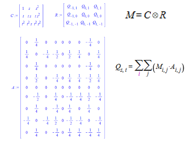
Q(s,t)

Note that the same formula applies first to the x coordinates, and then to the y coordinates and can work in any number of dimensions 2 or greater, Imagine that Q can be any of X, Y, Z component axis, and s and t vary continuously from -1..1... I'm not sure if there might be a notation using summations or matrices that makes this simpler and nicer to write, but maybe it's not that big of a deal when you can just write Q(s,t) to mean this in other formulas... It can also be fairly easily extended to volumes or higher dimensional objects using more variables than just s and t....

It's derived from my earlier post on the E_Bezier:
http://benpaulthurstonblog.blogspot.com/2015/12/ebezier.html...

One can derive something in a similar way from regular Beziers but then the mapping isn't conformal...

I made s and t vary from -1..1 so they can shrink to -delta +delta around a point on surface F for a sort of surface approximation, it can be shown that as delta shrinks to 0 in the limit the result is F at that point..Or to make the Q values closer and closer to surface F at a point to get a sort of parameterized surface derivative or tangent surface ( I think! I might explore that in a later post)... Also parameterization is a natural fit for conformal mappings because they are both scale and translation-invariant (also rotation)... A rectangle under a conformal mapping can be achieved by adding a coefficient multiplying one of or both t and s,.

I think maybe General Relativity might be simpler rewritten with this type of formula in mind, because it seems like the complicated thing is keeping all the axis components sorted out whereas this you can do each variable individually with the same formula, just a guess though I don't know that much about General Relativity...

**Matrix version**

Or using matrices instead of the row and column vector and the tensor product:

**Python Program**

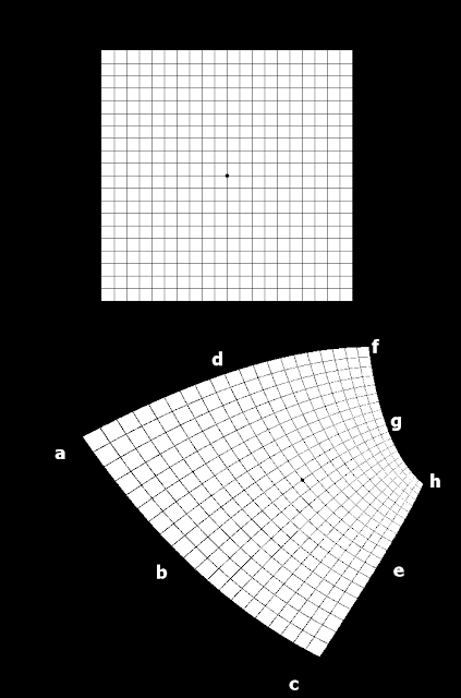
It's more convenient to use a bit different formula when doing things with computer images, ... It's the function q in the program below and the program takes any image of any size and maps it according to the following, there's also a variable for a value for oversampling; this one below is 2*x oversampled...: This map was actually made with the program, you can see the grid lines only ever cross at right angles, that's the conformal property...

**Python Code listing (using Pillow for python)**

from PIL import Image

def q(s,t,a,b,c,d,e,f,g,h):

    p = 1.0*((1/4)*b-(1/2)*s*b+(1/2)*s*s*b+(1/2)*t*t*d+(1/2)*t*d+(1/4)*e+(1/4)*g+

             t*t*s*s*((1/4)*g+(1/4)*b+(1/4)*d+(1/4)*e)-(1/2)*t*t*s*g+(1/2)*s*s*g+

             (1/2)*s*g-s*s*((1/4)*g+(1/4)*b+(1/4)*d+(1/4)*e)-t*t*((1/4)*g+(1/4)*b+

             (1/4)*d+(1/4)*e)-(1/2)*t*t*s*s*e+(1/2)*t*s*s*e+(1/4)*t*s*f+(1/4)*t*s*s*f+

             (1/4)*t*t*s*f+(1/4)*t*t*s*s*f-(1/4)*t*t*s*c-(1/4)*t*s*s*c+

             (1/4)*t*t*s*s*c+(1/4)*t*s*c-(1/2)*t*t*s*s*g-(1/2)*t*e+(1/2)*t*t*e-

             (1/2)*t*t*s*s*b+(1/2)*t*t*s*b+(1/4)*d-(1/2)*t*s*s*d-(1/2)*t*t*s*s*d+

             (1/4)*t*t*s*s*a-(1/4)*t*s*a-(1/4)*t*t*s*a+(1/4)*t*s*s*a-(1/4)*t*s*s*h+

             (1/4)*t*t*s*s*h+(1/4)*t*t*s*h-(1/4)*t*s*h)

    return p

def main():

    grid = Image.open("grid.png")

    output = Image.new("RGB", [700, 1200])

    w, h = grid.size[0], grid.size[1]

    c = [[116, 724],[288,926],[477,1059],[354,622],[579,897], \

         [552,588],[582,717],[634,796]]

    print(w,h)

    oversample = 2

    for i in range(0, oversample*w):

        for j in range(0, oversample*h):

            

            s = (2.0/w)*(i/oversample*1.0)-1

            t = -((2.0/h)*(j/oversample*1.0)-1)

            color = grid.getpixel((i/oversample*1.0,j/oversample*1.0))

            px = q(s,t,c[0][0], c[1][0], c[2][0], c[3][0], c[4][0], c[5][0], c[6][0], c[7][0])

            py = q(s,t,c[0][1], c[1][1], c[2][1], c[3][1], c[4][1], c[5][1], c[6][1], c[7][1])

            px = int(px)

            py = int(py)

            try:

                output.putpixel((px,py), (color, color, color))

            except:

                print((i,j), (px, py))

    output.save("conformal.png")

main()

**Chaining q(s,t)**

It's also pretty straight forward to chain for example a seamless texture to make a warped texture band...

Interesting non-regular pentagon

Questions for further study: Can you tile the plane with these? Are the angles inside the points of the star the same? Is the center pentagon made by the star regular?

Tr(n)^2+Tr(n+1)^2=Tr((Tri(n) + Tri(n+1)) for triangular numbers

I found this about the triangular numbers, also known as the number of distinct pairwise combinations of n items or the sum of the first n of 1,2,3,4,... this wasn't listed on the Encyclopedia of Integer sequences... , The formula for a triangular number is:

I found that:

Provable easily by substituting the formula for Tri in each side:

MacLaurin Generating Function

Exponential generating functions follow the form:

I was considering a modification of this structure to read:

Where f_n_(x) at x is both the sequence of coefficients to find the generating function for and the nth derivative at x following the convention of the MacLaurin Series for a function...
If we call this a MacLaurin Generating Function, then we can get some interesting series at x=1...

It continues after 0,1,2,3 with 8,10,54... and I've just learned that these are the Lehmer-Comtet numbers: Lehmer-Comtet

Now we can see what other of these types of series might have simple MacLaurin generating functions, below is if you use x^(2*x)

Maybe not as complicated as it looks when you substitute in x=1 that last 7th derivative is:

Still pretty complicated but the non power of 2 numbers look to be related to multiples of factorials?

The series 1, 2, 6, 18, 64, 220, 888 is not in the Encyclopedia of Integer sequences, but looks interesting! In fact Alois P. Heinz has already pointed out that the exponential generating function for x^2*x is x^2*x itself!

Factorial sum Maple doesn't know

Considering the sum:

But it's clear this sum should be equal to one, consider the first 7 terms:

If we were to increase the last coefficient by 1 it is exactly unity:

This is because 8/8! is 7! which adds one more 7! to 6/7! to make 7/7! which is 6!, etc.. until you have 1/2! plus 1/2! equaling 1...

It's kind of interesting to think what function would have this as it's MacLaurin series, that at f=1 it is 0, and the first derivative there is 1, and every successive derivative is 1 more than the one before it...
It actually is (x^x)-1, see:

Alternate numbering system

Just considering this series, here are the first 9 terms:

Where the next coefficient is chosen so the sum is as large as it can be not exceeding 1... The growth of the coefficients  can be solved for by noting the next term should by multiplied by some a so that it is as large as the previous term when it has a coefficient of 1...

Plotted it is linear:

So I've noticed that this series is basically as efficient for writing any number between 0 and 1 with regards to number of decimal digits as decimal itself is! By the pigeon hole principle no series can be better for getting k decimal digits than the decimal series a1/10 + a2/100...

Quadratic rule of eighths

This follows simply by substituting 1/4 and 3/4 into the E_Bezier formula from last post...