analytics

Thursday, November 22, 2012

Golden matrices

I noticed if you alternate between multiplying between these two matrices B and C:

Then when you multiply by the [1,1] vector you end up with a vector of successive terms of the Fibonnaci sequence. If you do more and more multiplications before finally multiplying by [1,1] you will get closer and closer to the golden ratio. 

If you instead of [1,1] multiply the resulting matrix by something else such as [2,15]:

Note that the resulting vector's x and y value are still in the golden ratio. 


Wednesday, November 21, 2012

Dependent suspension

I thought of this idea for the frame of a bike or a car that is designed so when you go over bumps the frame stays as level as possible.


Sorry for the poor drawing but it is basically a suspension that links the front and back wheels up and down motion in reverse, so when the front goes up relative to the frame the back extends relative to the frame so overall the frame stays at the same inclination. 


Monday, November 12, 2012

$ and # operators

I'm considering an operator that looks like this:


This grid means for instance 9$3 = 33 and 3$9 = 33 and 3$(-9) = -33 and -3$(-9) = 33 and -3$(9) = -33 etc. In general:
a$b = b$a =(-b$-a) = (-a$-b) =  -(-b$a) = -(b$-a) = -(-a$b) = -(a$-b)

An interesting feature is that c = a$b for a unique pair of a and b. For instance 30 is 6$7 or -6$-7 and there is no other way to produce 30 from a pair of a and b, aka b and a.

The operation is transitive over addition:
a$(b+c) = a$b + a$c

but it is not commutative:
a$(b$c) != a$(b$c)

a$b is not  f(a,b,+,-,*,/)
simply because x$x = x^2 and x$0 = x
the only polynomial with rational coefficients that equals x^2 is x^2 itself and x*0 is 0 not x.

So in a way f(a,b,+,-,*,/,$) extends the usual algebra.

Every positive integer can form a binary tree like this:
30 = 6$7
but 6 is 2$3 and 7 is 1$5
2 and 3 are both 1$2 and 1$3
((1$2)$(1$3))$(1$4)
the 1's can be removed.
(2$3)$5

Two obvious extensions of the idea are to define $ over the rationals which looks to be possible as $ has nice continuity properties, for instance it is always increasing in the a and b directions. Also to make another operator say, #, that acts as the inverse of $. for instance (a$b)#a = b and (a$b)#b = a.


Saturday, November 10, 2012

Force ratios in Parametric Kinematics

Suppose you have you a part of a machine is following a parametric curve in space...
And another part is following a different curve in space...
The force ratio is just the ratio of the magnitude of the derivatives of both curves. 

Starting with a simple example... 
Say something is connecting a part of a machine moving from A to B and another part moving from C to D. The machine happens to be a ramp and a rope but a ramp is just probably the simplest machine. The two motions can be parameterized like so:

The distance from C to A is 30.06 and we'd like that distance between the two points on the curves to stay constant so...
Now we can solve for s in terms of t. 

Now R becomes:
The magnitude of the derivative of this equation is:
And the magnitude of the derivative of Q is 5. 
Since the output speed is slower, at 96%, the force on the object on the ramp has increased, via the action of the ramp as a machine. This means that it would require more force to stop the part of the machine from going along R then it would to stop the part moving along Q. 
Another example:
In the last blog post I calculated the motion of P4 for a crank length of 1 and a Coupler length of 5 to be:
Of course R2 is parameterized as:

The derivative of the first is: 
in the y direction and 0 in the x direction. so this is also the total magnitude of the derivative. 
The magnitude of the derivative of B is:

So the ratio of the two is:


A graph of it looks like:


Friday, November 9, 2012

Parametric Linkage Kinematics


Considering a machine like this:
As the point on the unit circle R2 goes around the block P4 slides up and down in it's channel.
Most treatments I've read say the follower will move up and down as a sine wave, but it's possible to be more exact...
 Let's say for example it's a unit circle centered at the origin and the channel is on the y axis...

First the point on the circle is parameterized like so:

Now parameterize with the same parameter the motion of the block P4:
This means the block is not moving in the x direction and it is moving some function f(t) in the y direction. 
Also, let's say the length of the coupler is 5. Then we know that the distance between C and P is 5 or:

Now we can solve for f(t) which ends up having 2 solutions. 

One of these corresponds to P arranged above the circle and the other below. Not the difference between these solutions and a sine wave... 

Another example might be the four bar linkage:
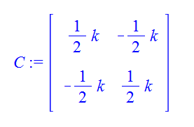
We can parameterize point B. 


where k(1), k(2), etc.  are the lengths of the connectors of A,B, C, D. 
 C is also parameterized but in general it will be to a different variable s and if A is at the origin then D will be offset to a point (x,y). 


The distance between B and C is k2 so:

Let's say k1 was 3, k2 = 4, and k3 =5 and (x,y) is the point (3,2)
then 
It's messy,but on a computer this can be solved for s and plugged back into the parametric equation for point C. Here's an animation of how C moves as T goes linearly from 0 to 2*pi. 


This animation shows the possible range of C, which is along a circle, though an anomaly in the graph shows a jump from one point on the circle to another. 


Thursday, November 8, 2012

heron matrix

I found this formula for finding the area of a triangle of sides length a,b,c; basically I started with Heron's formula and found a matrix multiplication that produces what would ordinarily be under the square root.

(After you add all the cells in the resultant matrix)

Tuesday, November 6, 2012

Deriving a cooling matrix from Newton's Law of Cooling

This is an improvement on the last blog entry inspired by a suggestion from Dr. Rose.

Suppose you start with a grid of temperatures like this:

Newton's law of cooling says that an object cools at a rate proportional to the difference of temperatures between itself and its surroundings.
So just considering that this grid is connected everywhere but the diagonals, the cell with starting temperature a would be expected to cool like:
T(new) = a-(k*(b-a) + k(c-a))/2
In other words the value of a cools proportionally to the average of the differences between it's surroundings and itself.

I introduce this matrix:


Now consider the following procedure: A-(A*C+C*A)


So the top left cell and the others are equal to our formula:
T(new) = a-(k*(b-a) + k(c-a))/2
 = a- ((.5)*kb -.5ka) +(.5kc - .5ka)
then grouping the ka terms
=a-ka +.5kb +.5kc

Now as for the fact that this doesn't consider cooling across the diagonals, what will happen is after one time step the top left corner and the bottom left corner cool towards each other, and then the next time step the new temperature in the bottom left corner will cool the bottom right corner, so actually information from the top left corner does reach the bottom right corner it just takes an extra step.


Also the sum of the four cells conserves the total temperature:


Sunday, November 4, 2012

Cooling matrix

Suppose you have a grid of temperatures such as:
I found this matrix C:
The interesting thing about C is when you do this operation: 
(matrix multiplication)
For the example matrix I gave A, this gives: 
The sum of all of these entries is exactly the same as the sum of all the entries in matrix A! 

If you look at matrix A and the resultant matrix you can see that every cell gets closer to the average value of all the entries in the matrix, which is what you would expect from a grid of temperatures settling into an average temperature. 

Let's look at the bottom right cell in A, that starts off at 7 and goes to 4.875, another application of the matrix multiplication with C gives: 
7
4.875
4.1406
3.83
3.673
3.584
3.531
3.498
3.478
...

You can see it is is sort of exponentially decaying to the average temperature of 3.444